35 Numerical differential equations

Numerical methods for ordinary differential equations are methods used to find numerical approximations to the solutions of ordinary differential equations (ODEs). Their use is also known as "numerical integration", although this term can also refer to the computation of integrals.

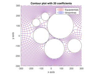
The analytic element method (AEM) is a numerical method used for the solution of partial differential equations. It was initially developed by O.D.L. Strack at the University of Minnesota. It is similar in nature to the boundary element method (BEM), as it does not rely upon discretization of volumes or areas in the modeled system; only internal and external boundaries are discretized. One of the primary distinctions between AEM and BEMs is that the boundary integrals are calculated analytically.

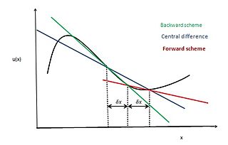
In applied mathematics, the central differencing scheme is a finite difference method that optimizes the approximation for the differential operator in the central node of the considered patch and provides numerical solutions to differential equations. It is one of the schemes used to solve the integrated convection–diffusion equation and to calculate the transported property Φ at the e and w faces, where e and w are short for east and west. The method's advantages are that it is easy to understand and implement, at least for simple material relations; and that its convergence rate is faster than some other finite differencing methods, such as forward and backward differencing. The right side of the convection-diffusion equation, which basically highlights the diffusion terms, can be represented using central difference approximation. To simplify the solution and analysis, linear interpolation can be used logically to compute the cell face values for the left side of this equation, which is nothing but the convective terms. Therefore, cell face values of property for a uniform grid can be written as:

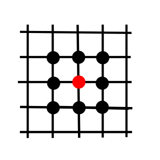
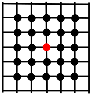
In mathematics, especially in the areas of numerical analysis called numerical partial differential equations, a compact stencil is a type of stencil that uses only nine nodes for its discretization method in two dimensions. It uses only the center node and the adjacent nodes. For any structured grid utilizing a compact stencil in 1, 2, or 3 dimensions the maximum number of nodes is 3, 9, or 27 respectively. Compact stencils may be compared to non-compact stencils. Compact stencils are currently implemented in many partial differential equation solvers, including several in the topics of CFD, FEA, and other mathematical solvers relating to PDE's.

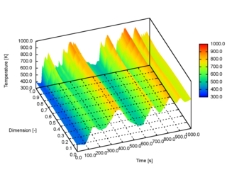
In numerical analysis, the Crank–Nicolson method is a finite difference method used for numerically solving the heat equation and similar partial differential equations. It is a second-order method in time. It is implicit in time and can be written as an implicit Runge–Kutta method, and it is numerically stable. The method was developed by John Crank and Phyllis Nicolson in the mid 20th century.

In mathematics and computational science, the Euler method is a first-order numerical procedure for solving ordinary differential equations (ODEs) with a given initial value. It is the most basic explicit method for numerical integration of ordinary differential equations and is the simplest Runge–Kutta method. The Euler method is named after Leonhard Euler, who treated it in his book Institutionum calculi integralis.

The extended discrete element method (XDEM) is a numerical technique that extends the dynamics of granular material or particles as described through the classical discrete element method (DEM) by additional properties such as the thermodynamic state, stress/strain or electro-magnetic field for each particle. Contrary to a continuum mechanics concept, the XDEM aims at resolving the particulate phase with its various processes attached to the particles. While the discrete element method predicts position and orientation in space and time for each particle, the extended discrete element method additionally estimates properties such as internal temperature and/or species distribution or mechanical impact with structures.

The extended finite element method (XFEM), is a numerical technique based on the generalized finite element method (GFEM) and the partition of unity method (PUM). It extends the classical finite element method (FEM) approach by enriching the solution space for solutions to differential equations with discontinuous functions.

The fast marching method is a numerical method created by James Sethian for solving boundary value problems of the Eikonal equation:

In numerical analysis, finite-difference methods (FDM) are a class of numerical techniques for solving differential equations by approximating derivatives with finite differences. Both the spatial domain and time interval are discretized, or broken into a finite number of steps, and the value of the solution at these discrete points is approximated by solving algebraic equations containing finite differences and values from nearby points.

The finite element method (FEM) is the most widely used method for solving problems of engineering and mathematical models. Typical problem areas of interest include the traditional fields of structural analysis, heat transfer, fluid flow, mass transport, and electromagnetic potential. The FEM is a particular numerical method for solving partial differential equations in two or three space variables. To solve a problem, the FEM subdivides a large system into smaller, simpler parts that are called finite elements. This is achieved by a particular space discretization in the space dimensions, which is implemented by the construction of a mesh of the object: the numerical domain for the solution, which has a finite number of points. The finite element method formulation of a boundary value problem finally results in a system of algebraic equations. The method approximates the unknown function over the domain. The simple equations that model these finite elements are then assembled into a larger system of equations that models the entire problem. The FEM then uses variational methods from the calculus of variations to approximate a solution by minimizing an associated error function.

The dynamic design analysis method (DDAM) is a US Navy-developed analytical procedure for evaluating the design of equipment subject to dynamic loading caused by underwater explosions (UNDEX). The analysis uses a form of shock spectrum analysis that estimates the dynamic response of a component to shock loading caused by the sudden movement of a naval vessel. The analytical process simulates the interaction between the shock-loaded component and its fixed structure, and it is a standard naval engineering procedure for shipboard structural dynamics.

The finite volume method (FVM) is a method for representing and evaluating partial differential equations in the form of algebraic equations. In the finite volume method, volume integrals in a partial differential equation that contain a divergence term are converted to surface integrals, using the divergence theorem. These terms are then evaluated as fluxes at the surfaces of each finite volume. Because the flux entering a given volume is identical to that leaving the adjacent volume, these methods are conservative. Another advantage of the finite volume method is that it is easily formulated to allow for unstructured meshes. The method is used in many computational fluid dynamics packages. "Finite volume" refers to the small volume surrounding each node point on a mesh.

Finite-difference time-domain (FDTD) or Yee's method is a numerical analysis technique used for modeling computational electrodynamics. Since it is a time-domain method, FDTD solutions can cover a wide frequency range with a single simulation run, and treat nonlinear material properties in a natural way.

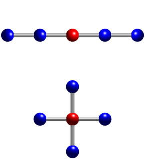
In numerical analysis, given a square grid in one or two dimensions, the five-point stencil of a point in the grid is a stencil made up of the point itself together with its four "neighbors". It is used to write finite difference approximations to derivatives at grid points. It is an example for numerical differentiation.

In mathematics, in the area of numerical analysis, Galerkin methods are a class of methods for converting a continuous operator problem to a discrete problem. In principle, it is the equivalent of applying the method of variation of parameters to a function space, by converting the equation to a weak formulation. Typically one then applies some constraints on the function space to characterize the space with a finite set of basis functions.

In numerical mathematics, the gradient discretisation method (GDM) is a framework which contains classical and recent numerical schemes for diffusion problems of various kinds: linear or non-linear, steady-state or time-dependent. The schemes may be conforming or non-conforming, and may rely on very general polygonal or polyhedral meshes.

High-resolution schemes are used in the numerical solution of partial differential equations where high accuracy is required in the presence of shocks or discontinuities. They have the following properties:Second- or higher-order spatial accuracy is obtained in smooth parts of the solution. Solutions are free from spurious oscillations or wiggles. High accuracy is obtained around shocks and discontinuities. The number of mesh points containing the wave is small compared with a first-order scheme with similar accuracy.

High-order compact finite difference schemes are used for solving third-order differential equations created during the study of obstacle boundary value problems. They have been shown to be highly accurate and efficient. They are constructed by modifying the second-order scheme that was developed by Noor and Al-Said in 2002. The convergence rate of the high-order compact scheme is third order, the second-order scheme is fourth order.

The infinite element method is a numerical method for solving problems of engineering and mathematical physics. It is a modification of finite element method. The method divides the domain concerned into infinitely many sections. In the first instance this results in an infinite set of equations, which is then reduced to a finite set. The method is commonly used to solve acoustic problems.

Mesh generation is the practice of creating a mesh, a subdivision of a continuous geometric space into discrete geometric and topological cells. Often these cells form a simplicial complex. Usually the cells partition the geometric input domain. Mesh cells are used as discrete local approximations of the larger domain. Meshes are created by computer algorithms, often with human guidance through a GUI, depending on the complexity of the domain and the type of mesh desired. The goal is to create a mesh that accurately captures the input domain geometry, with high-quality (well-shaped) cells, and without so many cells as to make subsequent calculations intractable. The mesh should also be fine in areas that are important for the subsequent calculations.

In the field of numerical analysis, meshfree methods are those that do not require connection between nodes of the simulation domain, i.e. a mesh, but are rather based on interaction of each node with all its neighbors. As a consequence, original extensive properties such as mass or kinetic energy are no longer assigned to mesh elements but rather to the single nodes. Meshfree methods enable the simulation of some otherwise difficult types of problems, at the cost of extra computing time and programming effort. The absence of a mesh allows Lagrangian simulations, in which the nodes can move according to the velocity field.

The method of lines is a technique for solving partial differential equations (PDEs) in which all but one dimension is discretized. MOL allows standard, general-purpose methods and software, developed for the numerical integration of ODEs and DAEs, to be used. Many integration routines have been developed over the years in many different programming languages, and some have been published as open source resources.

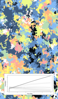
Microscale models form a broad class of computational models that simulate fine-scale details, in contrast with macroscale models, which amalgamate details into select categories. Microscale and macroscale models can be used together to understand different aspects of the same problem.

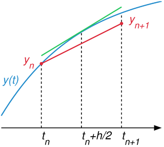
In numerical analysis, a branch of applied mathematics, the midpoint method is a one-step method for numerically solving the differential equation,.

The natural element method (NEM) is a meshless method to solve partial differential equation, where the elements do not have a predefined shape as in the finite element method, but depend on the geometry.

In numerical mathematics, a non-compact stencil is a type of discretization method, where any node surrounding the node of interest may be used in the calculation. Its computational time grows with an increase of layers of nodes used. Non-compact stencils may be compared to Compact stencils.

In computational mathematics, numerical dispersion is a difficulty with computer simulations of continua wherein the simulated medium exhibits a higher dispersivity than the true medium. This phenomenon can be particularly egregious when the system should not be dispersive at all, for example a fluid acquiring some spurious dispersion in a numerical model.

Partial element equivalent circuit method (PEEC) is partial inductance calculation used for interconnect problems from early 1970s which is used for numerical modeling of electromagnetic (EM) properties. The transition from a design tool to the full wave method involves the capacitance representation, the inclusion of time retardation and the dielectric formulation. Using the PEEC method, the problem will be transferred from the electromagnetic domain to the circuit domain where conventional SPICE-like circuit solvers can be employed to analyze the equivalent circuit. By having the PEEC model one can easily include any electrical component e.g. passive components, sources, non-linear elements, ground, etc. to the model. Moreover, using the PEEC circuit, it is easy to exclude capacitive, inductive or resistive effects from the model when it is possible, in order to make the model smaller. As an example, in many application within power electronics, the magnetic field is a dominating factor over the electric field due to the high current in the systems. Therefore, the model can be simplified by just neglecting capacitive couplings in the model which can simply be done by excluding the capacitors from the PEEC model.

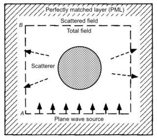
A perfectly matched layer (PML) is an artificial absorbing layer for wave equations, commonly used to truncate computational regions in numerical methods to simulate problems with open boundaries, especially in the FDTD and FE methods. The key property of a PML that distinguishes it from an ordinary absorbing material is that it is designed so that waves incident upon the PML from a non-PML medium do not reflect at the interface—this property allows the PML to strongly absorb outgoing waves from the interior of a computational region without reflecting them back into the interior.

In numerical analysis, the Runge–Kutta methods are a family of implicit and explicit iterative methods, which include the well-known routine called the Euler Method, used in temporal discretization for the approximate solutions of ordinary differential equations. These methods were developed around 1900 by the German mathematicians Carl Runge and Wilhelm Kutta.

In numerical analysis, the singular boundary method (SBM) belongs to a family of meshless boundary collocation techniques which include the method of fundamental solutions (MFS), boundary knot method (BKM), regularized meshless method (RMM), boundary particle method (BPM), modified MFS, and so on. This family of strong-form collocation methods is designed to avoid singular numerical integration and mesh generation in the traditional boundary element method (BEM) in the numerical solution of boundary value problems with boundary nodes, in which a fundamental solution of the governing equation is explicitly known.

Smoothed-particle hydrodynamics (SPH) is a computational method used for simulating the mechanics of continuum media, such as solid mechanics and fluid flows. It was developed by Gingold and Monaghan and Lucy in 1977, initially for astrophysical problems. It has been used in many fields of research, including astrophysics, ballistics, volcanology, and oceanography. It is a meshfree Lagrangian method, and the resolution of the method can easily be adjusted with respect to variables such as density.

In mathematics, especially the areas of numerical analysis concentrating on the numerical solution of partial differential equations, a stencil is a geometric arrangement of a nodal group that relate to the point of interest by using a numerical approximation routine. Stencils are the basis for many algorithms to numerically solve partial differential equations (PDE). Two examples of stencils are the five-point stencil and the Crank–Nicolson method stencil.

In computational fluid dynamics, the volume of fluid (VOF) method is a free-surface modelling technique, i.e. a numerical technique for tracking and locating the free surface. It belongs to the class of Eulerian methods which are characterized by a mesh that is either stationary or is moving in a certain prescribed manner to accommodate the evolving shape of the interface. As such, VOF is an advection scheme—a numerical recipe that allows the programmer to track the shape and position of the interface, but it is not a standalone flow solving algorithm. The Navier–Stokes equations describing the motion of the flow have to be solved separately. The same applies for all other advection algorithms.